
Getting Started
A Bayesian network (BN) is used to model a domain containing uncertainty in some manner. In the past, the term causal probabilistic networks have been used. A BN is a directed acyclic graph (DAG) where each node represents a random variable. Each node contains the states of the random variable it represents and a conditional probability table (CPT) or in more general terms a conditional probability function (CPF). The CPT of a node contains probabilities of the node being in a specific state given the states of its parents. The following example demonstrates what all this means.
The Apple Tree Example
In this example, the domain is a small apple plantation belonging to Jack Fletcher (let's call him Apple Jack). One day Apple Jack discovers that his finest apple tree is losing its leaves. Now, he wants to know why this is happening. He knows that if the tree is dry (caused by a drought) there is no mystery - it is very common for trees to lose their leaves during a drought. On the other hand the loosing of leaves can be an indication of disease.
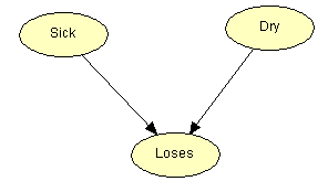
Figure 1: BN representing the domain of the Apple Jack problem.
The BN in figure 1 models that there is a causal dependency from Sick to Loses and from Dry to Loses. This is represented by the two arrows.
When there is a causal dependency from one node A to another node B, we expect that when A is in a certain state this has impact on the state of B. One should be careful when modeling the causal dependencies in a BN. Sometimes it is not quite obvious which direction an arrow should have. E.g. in our example we say that there is a causal arrow from Sick to Loses because when a tree is sick this might cause the tree to lose its leaves. But could we not say that when the tree loses its leaves, it might be sick and turn the arrow in the other direction? No, we cannot! It is the sickness that causes the lost leaves and not the lost leaves that cause the sickness.
Use the web form below to reason about the apple trees using this model.
| Loses Leaves? |
| Sick? | Probability | No | Yes |
In figure 1, we have the graphical representation of the BN. However, this is only what we call the qualitative representation of the BN. Before we can call it a BN, we need to specify the quantitative representation.
The quantitative representation of a BN is the set of CPTs of the nodes. Table 1, 2, and 3 show the CPT of the three nodes in the BN of figure 1.
|
Sick="sick" |
Sick="not" |
|
0.1 |
0.9 |
Table 1: P(Sick)
|
Dry="dry" |
Dry="not" |
|
0.1 |
0.9 |
Table 2: P(Dry)
|
|
Dry="dry" |
Dry="not" |
||
|
Sick="sick" |
Sick="not" |
Sick="sick" |
Sick="not" |
|
|
Losses="yes" |
0.95 |
0.85 |
0.90 |
0.02 |
|
Losses="no" |
0.05 |
0.15 |
0.10 |
0.98 |
Table 3: P(Losses | Sick, Dry)
Note that all three tables show the probability of a node being in a specific state depending on the states of its parent nodes but since Sick and Dry do not have any parent nodes, tables 1 and 2 are not conditioned by anything.