
Simple Bio Tracability Example
Gary Barker, IFR developed this example. The example is taken from this source
A Bayesian network is a compact model representation used for reasoning when a considerable amount of uncertainty is associated with the information that quantifies a system (i.e., a food chain). Such a model includes steps in the chain and processes along the chain, together with prior probability distributions on these steps and conditional probability distributions describing dependencies. A Bayesian network facilitates inference, i.e., it supports tracing. Figure 1 shows a limited-memory influence diagram representation of the problem domain called SimpleTrace.
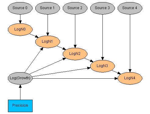
Figure 1: The SimpleTrace network.
The SimpleTrace network represents a finite chain of events with five identified (observable) elements i=0,4. At each stage of the chain an agent has a concentration Ni (The logarithm, LogNi, is the representative random variable). At each stage there is an uncertain source of agent with a fixed concentration 0.1. Boolean variables, Si, quatify the sources - all sources have prior probability 0.005.
Between consequtive elements in the chain finite concentrations of agent grow with according to an uncertain growth factor, in the range 1 - 100, expressed as log(Ni+1/Ni) ~ Beta(m,m,0,2). (In the network represenattion concentrations Ni < 0.01 are considered zero - the lowest concentration state acts as a sink). The growth factor is the same for all transitions. A decision node (Precision) can be used to choose m=200,20,1 (High, Medium, Low precision concerning the growth factor).
SimpleTrace illustrates a "trace" operation. Observations of the end point concentration, i.e. evidence entered at LogN4, provides posterior belief concerning the sources (source strengths). The ability to 'identify' a source as the origin of observed agents (i.e. "trace") depends on the decision concerning the precision of the growth factor.
We have five time-steps in the food chain; every time-step is characterized by a population-distribution of a pathogen (LogN0 to LogN4). At every time-step we have a potential source of contamination (Source 0 to 4). Every population size only depends on the previous polulation size and on an element of growth. The latter is express by the growth factor. We assume that we can only measure the population size at the last time-step.
Demonstration of the model
Select Growth Precision
Enter the measured value (possible values are between -3 and 7.25)
Analysis Results
The purpose is to identify the most likely source of a contamination.| Possible Source | Probability | Probability (bar view) |
| Source 0: | ||
| Source 1: | ||
| Source 2: | ||
| Source 3: | ||
| Source 4: |
When we using the above web form enter the observation that the contamination at the last time-step, Log4N, is 1.35, the information propagation computed by HUGIN updates the beliefs on the initial contamination. It can be seen that the contamination probably occurred at time-step 2. There is a probability of 94.96% that the contamination came from Source 2.